MEL-GENERALIZED CEPSTRAL ANALYSIS — A UNIFIED APPROACH TO SPEECH SPECTRAL ESTIMATION

Introduction:

As per the source-filter model,we can see our speech production system as excitation at the glottis passing through a acoustic filter(vocal tract). As you see the below figure the excitation is approximately a impulse train(voiced speech) and the filter has smooth frequency response depending on the what phoneme is been spoken(vocal tract shape). In time domain the impulse train is convoluted with the filter impulse response to get the speech(similarly multiplication in time domain).

Figure 1: Source-Filter Demo on 25 ms speech: Left-Top:source impulse train,Right-Top: frequency response of impulse train with hamming window,Middle: impulse and frequency response of the filter.

The main goal of the Spectral Estimation technique is to recover the frequency response of the filter(Middle-left: $H(e^{j\omega})$ ) or parametric (compressed) version from the speech spectrum(Bottom-left). As you can see that the speech spectrum is disturbed by the source signal. But the envelope of the spectrum could be good representation of the $H(e^{j\omega})$ .There is a lot methods proposed to estimate the parameters of both source and filter.Here we focus on one general method that tries to estimate the parameters of the filter/envelope of the spectrum(like frequency response/impulse response).

The parameterization of the filter is useful in compressing the frequency response of the filter. This will be help reducing the bandwidth required in communication or modelling speech with less number of parameters for various purpose like speech recognition,text to speech etc.

In this article we explore briefly about some of the famous spectral estimation technique used speech processing, disadvantages of them and how the Mel-Generalized Cepstral estimation over comes that disadvantages. This article is mainly focused on understanding intuitively/graphically with less math. The mathematical details can found the respective PDF links given.

Review of some of the methods:

Please refer the references for more details,here i just give intuitive explanation of each method.

Linear Predictive Coefficients(LPC): In this method the $H(e^{j\omega})$ by a all-pole model(there are only poles in the filter). $H(e^{j\omega})$ = $\sum_{m=1}^{M}a_{m}z^{-m}$ . This will start failing if the system is not all-pole,for instance like nasals that has zeros. The LPC will not be able to recover the filter response in the place of zeros. As shown in the Figure 2. Refer these links to understanding the estimation of the coefficients(a)[1][2][3].
Cepstrum: Since the LPC cannot recover the $H(e^{j\omega})$ when there are zeros in the spectrum. The zeros cause the frequency response to have low value at some frequency bins. So we need a method where we can expand these values to higher values like logarithm. In Cepstrum method the $ln(H(e^{j\omega}))$ is represented by the all-pole model( $ln(H(e^{j\omega}))$ = $\sum_{m=1}^{M}a_{m}z^{-m}$ ). The log-compression causes the pole and zero values to comparable and zeros also can be represented efficiently. But if there are shape peaks(the poles closer to unit circle) in the $H(e^{j\omega})$ ,this method compress that peak.So it cannot represent the sharp peaks properly.
Mel-Scale: So-far we saw only representing the ,but equally-well in all frequency region. As the order M increases, both methods starts approximating the spectrum more accurately[*]. But the human ear has higher resolution at low-frequency region and low-resolution at high-frequency regions. So it better to represent the accurately in low-frequency than the higher frequency. So spectrum can be warped(more number of DFT points at lower-frequency than higher frequency) and represented by one of the above two methods. The methods are called as Mel-LPC and Mel-Cepstrum.
- Mel-LPC: $H(e^{j\omega})$ = $\sum_{m=1}^{M}a_{m}\hat{z}^{-m}$
- Mel-Cepstrum:(= )
  - where $\hat{z}= \frac {z^{-1}-\alpha}{1-\alpha z^{-1}}$ and $\alpha$ controls the trade off the resolution in high and low frequency.

[*]Accurately representing the speech spectrum is not our goal..! we have to represent the vocal tract response more accurately. Think about what happens as the M increases in case of LPC and cepstrum?

The diagrams shows a synthetic spectrum generated from poles at angle of 0,45,75 degrees. The radius of the pole/zero is mentioned in the plot. As per the diagram, the spectrum with zeros closer to unit circle(0.9) are better approximated by the cepstrum than the LPC. Similar the spectrum with poles are better approximated by LPC than cepstrum. If the spectrum has both zeros and poles, both methods are not able to approximate the spectrum. So Spectral estimation of speech by mel-generalized cepstral analysis and MEL-GENERALIZED CEPSTRAL ANALYSIS — A UNIFIED APPROACH TO SPEECH SPECTRAL ESTIMATION proposes a unified frame work where it can combine these methods.

allzeros

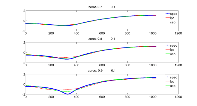
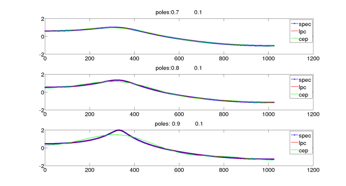
Figure 2: The comparison of the original spectrum and the approximated spectrum by LPC and cepstrum method for various pole or zero locations.

Spectral estimation of speech by Mel-generalized cepstral analysis:

The filter response $H(z)$ = $s_{\gamma}(\sum_{m=1}^{M}a_{m}\hat{z}^{-m}$ ). The $s_{\gamma}()$ and $\hat{z}$ will be defined later and the coefficients $a_{m}$ are found by minimizing the Unbiased estimation of log spectrum.

There are 5 main ideas of the papers as mentioned below:

1. Generalized logarithm:

As we saw earlier the LPC and cepstrum comparison where the compression of spectrum decides the approximation of the spectrum envelope. So we need a operator that decides the compression factor(denoted by $\gamma$ ). The generalized logarithm is defined as $s_{\gamma}(\omega)=\begin{cases} (\omega^{\gamma}-1)/\gamma & 0<\gamma\leq1\\ log(\omega) & \gamma=0 \end{cases}$

The $\gamma$ decides the compression factor, The $\gamma$ =1 the method is similar to the LPC and $\gamma$ =0 is cepstrum.

The synthetic spectrum after generalized logarithm transform for all-pole(top) and all-zero(bottom) systems.

As per the diagram the the different $\gamma$ value results in different compression.

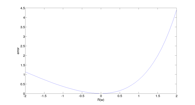
2. Unbiased estimation of log spectrum:

The error function minimized to estimate the coefficients is given by

$E=\frac{1}{2\pi}\intop_{-\pi}^{\pi}\left\{ e^{R(\omega)}-R(\omega)-1\right\} d\omega$

and $R(\omega)=I_{N}(\omega)-log(|H(e^{j\omega})|^{2}$ , where the $I_{N}$ is the windowed spectrum.

The error function is very crucial to estimate the envelope because this error function penalizes the +ve error less than the -ve error. The error function for $R(\omega)$ single dimension is shown below. As you see that the E is higher for -ve error than the +ve error. So that the envelope of spectrum is approximated.

This very helpful in the speech is because the envelope information in the spectrum is sampled by the pitch. So that the direct mean square error(penalized equally the +ve and -ve errors) is not preferred compared to the error mentioned above. The mean square allows both +ve error and -ve errors, but the actual envelope will not have any -ve errors.

error_fun

3. Warping:

The $\hat{z}$ is defined as $\hat{z}^{-1}=\frac{z^{-1}-\alpha}{1-\alpha z^{-1}}$ . As we discussed before the resolution at different scale can be different. The parameter $\alpha$ controls this resolution at different frequency. $\alpha>0$ will have high resolution at low frequency. The frequency transformation can be given by

$\tilde{\omega}=\beta(\omega)=tan^{-1}\left(\frac{(1-\alpha^{2})sin(\omega)}{(1+\alpha^{2})cos(\omega)-2\alpha}\right)$ .

proof can be found here.

4. Gain independent form:

The LPC( $\gamma$ =1) and Cepstrum( $\gamma$ =0) are doe not depends on the signal gain. But the generalized logarithmic definition makes the generalized coefficients depends on the signal gain. We need to change the basis of the representation of the $S_{\gamma}(H(\tilde{z}))$ . There are many method proposed to change the basis function so that the representation is independent of the gain form. One of the basis function is given below.

$H({z})=S_{\gamma}^{-1}(\sum_{m=0}^{M}b_{\gamma}(m)\Phi_{m}(z))=K.D({z})$

Where $\Phi_{m}(z)=\begin{cases} 1 & m=0\\ \frac{(1-\alpha^{2})z^{-1}}{1-\alpha z^{-1}}\tilde{z}^{-(m-1)} & m\geq1 \end{cases}$ . Now the gain is K and the coefficients representation is in the form of b. The relation between a & b can be found using above equation and the proof can be found here.

Given the above 4 ideas the representation(a or b) can be found by optimizing the error(E) with respect to a or b. If we consider optimizing with respect to b. substituting the basis change to the E and simplifying gives the simplified error function as shown below. The proof can be found here. $\epsilon=\frac{1}{2\pi}\int_{-\pi}^{\pi}\frac{I_{N}(\omega)}{|D(e^{j\omega})|^{2}}d\omega$ .

5. Direct synthesis filter from the coefficients:

As mentioned earlier the $H({z})=K.D({z})$ with $D({z})$ is defined completely by the coefficients “b”. So the $H({z})=\frac{Y({z})}{X({z})}$ and hence the coefficients “b” can be directly used as filter coefficients of the filter to get the required frequency response. Even though it is consequence of the point (4), It is important property of the representation that can synthesize back the signal unlike MFCC.

The optimization is performed using the gradient descent/newton method that needs first and second order derivatives. Its computation can be found here.

The other advantages of the method:

The error function is convex with respect to the coefficients b.(proof can be found here)
The coefficients of the synthesis filter is always stable(proof can be found here)

Simulations using different synthetic spectrum:

role of $\alpha$ :

As we discussed before the $\alpha$ decides the resolution of spectrum approximation at different frequency. To test this we consider the synthetic spectrum of there types of signal similar to linear chirp: decreasing frequency,constant frequency and increasing frequency in each row of the figure. The MGC is computed and reconstructed back the spectrum at different value of $\alpha$ ={0.35,0.0,-0.35},but $\gamma$ =0.

As shown in the diagram, In all spectrum shape the $\alpha$ >0 tends to fit the spectrum at low frequency than the high frequency compare to other $\alpha$ values. So depending on requirement of the problem the $\alpha$ can be selected to get the resolution at different frequencies.

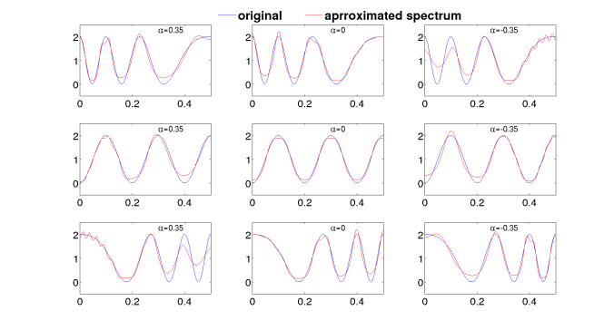
Spectrum approximation by 16th order MGC with different value of alpha and gamma=0 for different kind of variations at lower and higher frequency regions.

Do we really have fine control on all frequency resolution using a single parameter $\alpha$ ?

role of $\gamma$ :

As discussed before, the $\gamma$ controls the ability to fit the peaks of the spectrum. Here we consider three types of the spectrum with different sharpness of the peaks as shown in the diagram below. As you can see that the sharper the spectrum the the value of $\gamma$ closer to -1 fits better the spectrum. So we can decide the value of the $\gamma$ depending the system characteristics(AR/MA/ARMA).

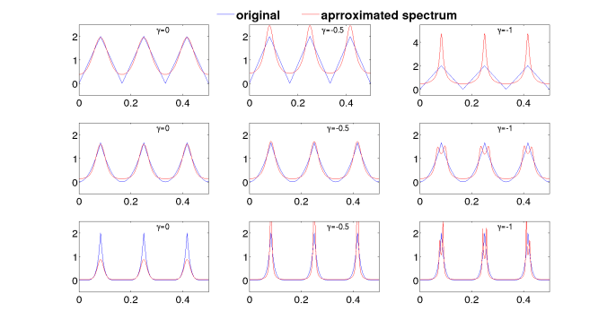
Spectrum approximation by 16th order MGC with different value of gamma and alpha=0

Similarly both $\gamma$ and $\alpha$ could be varied to fit the specification of the spectrum.

Discussion:

Even though we have the flexibility of controlling the spectrum approximation using MGCs. It has the following shortcomings.

The frequency resolution at given band cannot be increased compared to the out off band. This limitation is because of form of frequency warping is used in the method.The flexibility of this can be increased to have better control on frequency resolution.
The generalized log will compress all the bins of the spectrum depending on $\gamma$ value. It might be good idea have operation where is compress the different part of the spectrum by different factors,so that the both poles and zeros of the spectrum can be represented even more efficiently.
The value of $\gamma$ and $\alpha$ is fixed and there is no automatic way of determining based on the spectrum itself. So for highly non-stationary signal like speech the fixed value of $\gamma$ may not be good enough,but there are some perception based experiments that recommends some value of $\alpha$ for given sampling rate.

Achuth Rao M V

imagination is better than knowledge -Albert Einstein

MEL-GENERALIZED CEPSTRAL ANALYSIS — A UNIFIED APPROACH TO SPEECH SPECTRAL ESTIMATION