Hi Everyone,
In this article, we understand the paper “The Dual Form of Neural Networks Revisited: Connecting Test Time Predictions to Training Patterns via Spotlights of Attention.” Neural networks are widely used for various tasks. Still, their exact working of them is not fully understood. Multiple ways are proposed to understand the trained network, such as activation and weight visualization. In this paper, the authors explore an alternate method of understanding the neural network using the dual form of the neural network were they as the following question:
is it possible to point out exactly which training samples are the original sources of that specific output?
We use some of the equations directly from the paper. We try to discuss only some aspects of the article in detail. The title summarizes the main contributions perfectly as it can be listed as follows:
- How Unnormalized dot attention is a particular case of the linear layer and equivalence between the two.
- Write gradient descent (GD) update equation of the weight for both linear layer and the attention for the whole course of training.
- Show that the test prediction based on the final weight can be written as a linear combination of the error signal during the training.
The connection between linear layer and unnormalized dot product attention
The unnormalized dot attention can be defined as 
where 

If we consider a linear layer with parameter W with input 


The dual form of linear layer trained by gradient descent
The linear layer is the core of many neural networks, such as fully connected layers, convolutional neural nets, LSTM, and transformers. We focus on the parameter evolution of one linear layer (part of a big network). The loss function is L. The gradient descent update for the weight at 


where 

Given a test sample to the input layer 


where 


Important Remarks
- In the case of dual form, We need the inputs and the error signal for the entire training course to compute the test sample’s output. We just need one matrix multiplication in the direct linear layer. So the decision on the test input depends on the whole course of training and not just the final weight. This kind of a strange result, and we will try to illustrate it with examples in later sections.
- Note that the analysis is for a simple linear; it applies to all classes of neural nets with a linear layer (Almost all types of nets). The article considers general input, loss, and backpropagation errors.
Some more exciting remarks are found in the paper.
Illustrations:
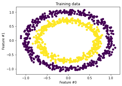
The paper illustrates results using various interesting examples for different tasks. In this article, we stick to a simple two-dimensional example of concentric circles shown in Fig. 1. The main idea is to visualize the connection between the training and the test data, as discussed above. We will see only a few examples; you regenerate and play around with different parameters in the colab notebook. If you have some questions, please post them in the comment section.
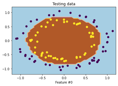
Let’s use a simple feedforward 3-layer network with 32 hidden dimensions with tanh activation. The network is trained for 50 epochs and achieves >90% accuracy (A straightforward problem anyway). The simple classification boundary and the test points are shown in Fig 2.
Lets a sample test point and compute the attention weights( 
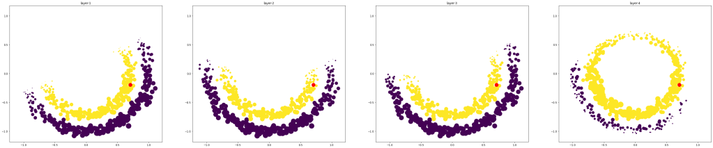
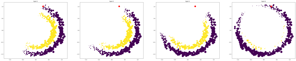
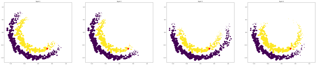
Three rows indicate the attention weights for three test points. Three columns indicate the attention weight computed from layer1-layer-4 respectively.
It is clear from the figure that the test predictions mainly depend on only a subset of the data. The attention weights are typically high around the test points, but it is not always the case. If the test point is well within the boundary, then the final layer output depends mainly on the data in only one class (rows 1 and 2). The points near the classification boundary rely on the training data from both classes.
Conclusion
The dual form of the linear layer is used to connect the test predictions to training data. It can be used in any neural network that has a linear layer. This can be used to explain the test prediction using the training data. The method can be computationally infeasible for some large models or data settings because it needs to store the whole history of training. Understanding the evolution of
