Similar ideas are applicable in case of Normalizing flows, You can find more details in another tutorial.
Variational Auto Encoder (VAE) is one of the famous generative models and applied for various unsupervised, semi-supervised tasks [1][2]. There is a lot of interesting ways to look at how it works [3]. But in this article, we try to develop the idea of the VAE just from the knowledge of elementary random process/probability.
First Let us look at the definition of the cumulative distribution functions (cdf) of a continues random variable X.

where 


But let us ask our self what happens if random variable (X) go through a transformation 

here we are assuming that the
Now think about what happens if the 


Now let us try to reverse the process, what happens if we start with random variable Y with the distribution Uni(0,1) and pass through a function 
It will be
…! (Think about it)
Now we know that if we know CDF (
Now we understand how we can generate random numbers from any distribution. Let us link it to VAE.
Let assume that we have a set of N-identical and independent samples

But there are two main questions:
- How do we make the distribution of y close to Uni(0,1)?
- What is the use of approximating
, we cannot generate the data from the generative models?
The first question is difficult in terms of learning/objective function of the neural network (issues like differentiability/backpropagation) and the second question is not answered by our solution.
So let us propose some other modification to this. Let us map from x to y and then map y to 
- Make the
- To make the generative process clear, we need to force the distribution of y to Uni(0,1).
The first objective is simple, we can use error like mean squared error or weighted mean squared error make the
But we can look the second objective in a slightly different way, Let us ask our self, can we generate the numbers from arbitrary distribution given the random number from a Gaussian distribution (z)?
The answer is simple, Let us the function g(z) map from Gaussian distribution to uniform distribution (u) and another function h(u) map from a uniform distribution to required distribution (x). The outline is given below.
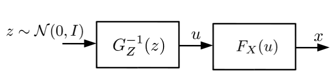
Generating data from the arbitrary distribution using the Gaussian distributed data. Where the distribution of u is a uniform distribution.
Here we assumed that simplest Gaussian distribution of zero mean and identity co covariance matrix. The overall function to generate a random variable from the distribution p(x) can be written as h(g(z)), where the distribution of z is Gaussian.
So now our whole process can be written as shown in the figure.
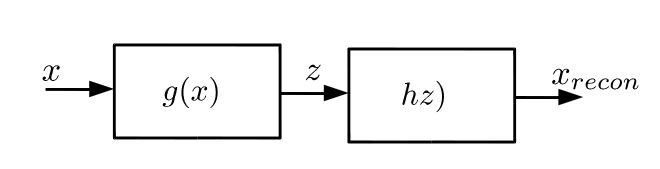
Our whole process block diagram
start with the data x and map it to a variable y using a function G(x) and map the y to 
So the overall objective sum of both the objectives:
![E(x, [latex]x_{recon}](https://s0.wp.com/latex.php?latex=E%28x%2C%C2%A0%5Blatex%5Dx_%7Brecon%7D&bg=ffffff&fg=444444&s=0&c=20201002)
We can see that the objective is exactly same as the VAE objective…!
The specific details of the implementation and the optimization can be found in the main paper [1]. Once the network is learned the data generated from the model is easy. First sample from the
In summary:
- Generating random numbers from the arbitrary distribution from Gaussian/Uniform distribution and the reverse process is known for a long time.
- Use neural network (theoretically approximate any function) to approximate the required function to map from one distribution to another.
- We saw the VAE is about reconstructing the data and forcing a distribution in a particular layer of a neural network can help in generating the data.
- The second term of the objective can be evaluated in closed form for Gaussian distribution and it allows for the backpropagation.
- There are some intricate details related to the learning process (finite sample size) is not discussed here.
Notes:
- Last two points in the summary are the main contribution of [1].
- The [1] approaches the problem from the Variational method framework. Where the true likelihood is lower bounded by the objective we just found above.
Have a great day.
-Achuth
Reference:
[1] Auto-Encoding Variational Bayes
[2]Tutorial on Variational Autoencoders
[3] Other nice blogs about VAE:
- https://jaan.io/what-is-variational-autoencoder-vae-tutorial/
- https://wiseodd.github.io/techblog/2016/12/10/variational-autoencoder/
- http://blog.fastforwardlabs.com/2016/08/12/introducing-variational-autoencoders-in-prose-and.html
- http://zhusuan.readthedocs.io/en/latest/vae.html
